Since 1800, when Carl Gauss published his magnum opus, the world has had the tools to explain ‘Probability Density’ or as we know it; “the Bell Curve”. We all remember Ferris Bueller’s day off when the high school teacher, played by Economist Ben Stein bored the class by explaining Arthur Laffer’s application of the bell curve to optimizing taxation……Anyone? Anyone?……Bueller? Bueller??
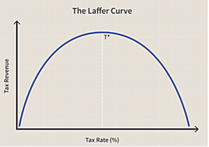
Such a simple concept! Can we apply it to other things? Laffer used this very simple concept to steer the nation to a theory that lowering tax rates can raise tax revenue. In short, businesses underperform when overtaxed as do households. But we need the taxes to pay for a variety of critical services. Laffer showed that there is an ‘appropriate’ rate of taxation. For the crime of being reasonable, he was immediately ignored!
For us in business, a variety of trade-offs are presented each day. Decisions are made as a function of need and the counterbalancing reward. When a business considers Cyber Security, a few simple thoughts can be used as a guidepost, as shown below.
Nearly all Cyber Security decisions can be considered starting with these three questions. Within Complex and large businesses, these three questions explode into hundreds of derivations, whereas a small business with a few computers may not need to answer many others. To illustrate this, I have developed the Cyber Security Risk vs. Expense Curve (credit to Mr. Laffer) which will guide us within the rest of this discussion.
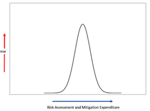
Figure 1
It may take a moment for this to sink in so let’s walk through this process. Your company is performing a risk assessment. It has been a while since one has been performed so the virus software that has been protecting your company needs to be upgraded to something new called Endpoint Detection & Response (EDR) (good idea) and the firewall is old, they are recommending something new and expensive but necessary, so the identified risks to your organization are quickly rising. The cost of the audit is escalating and once the risk assessment is complete you have spent X dollars and now need to spend more to mitigate these risks.
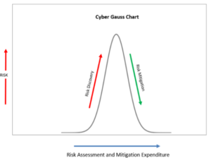
Figure 2
Here we are introduced to the Cyber-Gauss chart. As the discovery process progresses there are some early serious discoveries accelerating the amount of risk seen in the organization. As progress continues to mitigate these risks will require the expenditures to continue. The question we are trying to frame here is what is the proper amount of mitigation for the exposed risks?
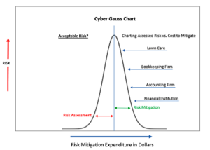
Figure 3
This is always a tough question. How much money do we budget to mitigate the risks? Or is the question really (and yes this is the right answer) that we should decide how much risk the organization should accept and mitigate the risks that are not acceptable? In our Cyber Gauss chart above we see that the approach we chose is to think of risk in proportion to the classification of the business. We appraise the composite risk and select the ones critical to the business as a mitigation and expense plan. Randomly I have selected four types of businesses that are requiring some degree of mitigation; however, it is assumed that all four of these companies have deployed similar infrastructure (for the sake of this exercise) would we spend the same to protect resources for all four types of businesses? This is where this curve is especially helpful. In a real exercise within a complex business taking the risk scores and assigning mitigation costs to each finding should provide a similar chart. Our cost of mitigation for a Lawn care company may only be the standard updates being confirmed, some EDR solution, and a backup strategy that is logged and reviewed by a third party. The Financial institution will find that there are many people looking over their shoulders and the level of acceptable risk is very low.
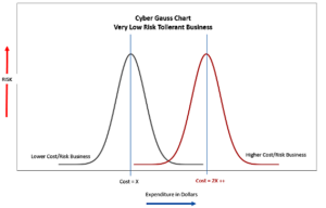
Figure 4
If your business is considered one where acceptable risk needs to be minimized and perhaps there are other organizations (Federal, State) looking over your shoulders, The assessments and mitigation cycles are continuous and multidimensional. Where there may be an IT assessment for the basic infrastructure and then an information security assessment which though similar will analyze processes and procedures for handling the information. A good way of understanding these types of complexity is with a chart that looks specifically at each risk assessment and separates the mitigation prior to understanding and properly assessing different mitigation approaches. The key takeaway is that risks are always found and the second team in is more specialized, will find risks and the cost of mitigation will stack.
In upcoming installments, depending on feedback, I may develop these further. However, I strongly recommend the use of these types of distributions to assist your team in visualizing the optimization of risk assessment mitigation.
For those of you that are disciplined mathematicians, my sincere apologies, I took many liberties to introduce this topic to those that are more IT focused.
Further reading:
Normal Curve using Excel 2010 (this is a very good toybox for those trying to unlock the concept of normalized distribution)
Carl Friedrich Gauss: Titan of Science
The Master Ben Stein with the Genius Director John Hughes: Boring Economics Teacher